Root Causing a Variance

Decomposing cost variances into rate and usage components

Free previewIntermediate

⏱️ About 45 min

A $1,600 cost overrun shows up on your report. Is it because labor rates spiked, or because the team worked more hours than planned? The total variance tells you there is a problem; it does not tell you why.

💡

The big idea: By splitting a total cost variance into a rate variance and a usage variance, you pinpoint whether the issue stems from unit costs or from quantity consumed.

🎯 By the end, you'll be able to

Calculate rate variance and usage variance from standard and actual figures
Explain why decomposing variances improves root cause analysis
Use a variance bridge to communicate drivers to stakeholders

📎 Helpful to know first

Familiarity with standard costs, actual costs, and basic EVM cost variance (CV).

Why Split a Variance?

A total cost variance tells you the magnitude of a deviation, but not its cause. When actual cost exceeds standard cost, the gap could be driven by higher unit rates, higher quantities consumed, or both. Splitting the variance isolates these two drivers.

\[ \Delta_{total} = (R_a - R_s)\,Q_a + (Q_a - Q_s)\,R_s \]

⚠️ Reading the Formula

The first term, (Ra - Rs) * Qa, isolates the rate variance: it holds quantity constant at the actual level and measures the cost impact of the rate difference. The second term, (Qa - Qs) * Rs, isolates the usage variance: it holds rate constant at the standard level and measures the cost impact of the quantity difference.

Unfavorable vs Favorable

When actual rate Ra exceeds standard rate Rs, the rate variance is unfavorable. When actual quantity Qa exceeds standard quantity Qs, the usage variance is unfavorable. A positive total variance indicates an overall cost overrun.

⚠️ The Variance Bridge

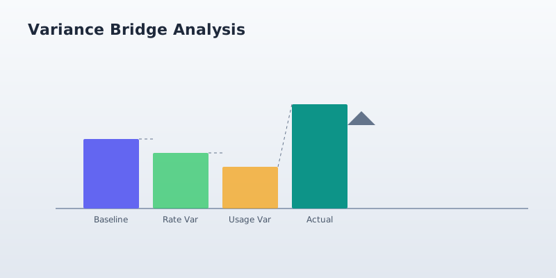
A variance bridge visually walks from standard cost (Rs * Qs) to actual cost (Ra * Qa) in two steps: first apply the rate change to reach an intermediate cost, then apply the usage change to reach actual cost. This makes the two drivers immediately clear to non-financial stakeholders.

🎮 Variance Bridge Simulator LIVE

Predict first: Adjust standard and actual rates and quantities to see how the total variance decomposes into rate and usage components.

The bridge shows the standard cost, the step up due to rate, the step up due to usage, and the actual cost.

📝 Worked example: A task has a standard rate of $50/hr and standard quantity of 100 hrs. The actual rate was $55/hr and actual quantity was 120 hrs. Decompose the total cost variance into rate and usage variances.

1. Rate variance = (Ra - Rs) * Qa = ($55 - $50) * 120 = $5 * 120 = $600
2. Usage variance = (Qa - Qs) * Rs = (120 - 100) * $50 = 20 * $50 = $1000
3. Total variance = Rate + Usage = $600 + $1000 = $1600 unfavorable.

✓ Rate variance = $600, Usage variance = $1000, Total variance = $1600 unfavorable.

✏️ Practice: Given Rs=$40, Ra=$45, Qs=200, Qa=180, calculate the rate variance.

💡 Hint

Rate variance = (Ra - Rs) * Qa. Subtract the standard rate from the actual rate, then multiply by the actual quantity.

Answer

900

Check your understanding

1. Using the figures Rs=$50, Ra=$55, Qs=100, Qa=120, what is the total cost variance?

Total variance = Rate variance ($600) + Usage variance ($1000) = $1600.

2. Why decompose a total cost variance into rate and usage components?

Decomposition isolates the root cause, telling you whether to negotiate rates or improve efficiency.

✅ Key takeaways

Total variance = Rate variance + Usage variance
Rate variance = (Ra - Rs) * Qa isolates the unit cost driver
Usage variance = (Qa - Qs) * Rs isolates the quantity driver
Splitting variances enables targeted root cause analysis

➡️ Now that you can diagnose why a variance occurred, the next step is learning how to formally adjust the baseline when scope changes are approved.

Ready for the next step? Back to the course outline →