
Populations vs Samples
The whole group you care about, the slice you actually measure, and why the gap between them is the heart of statistics.
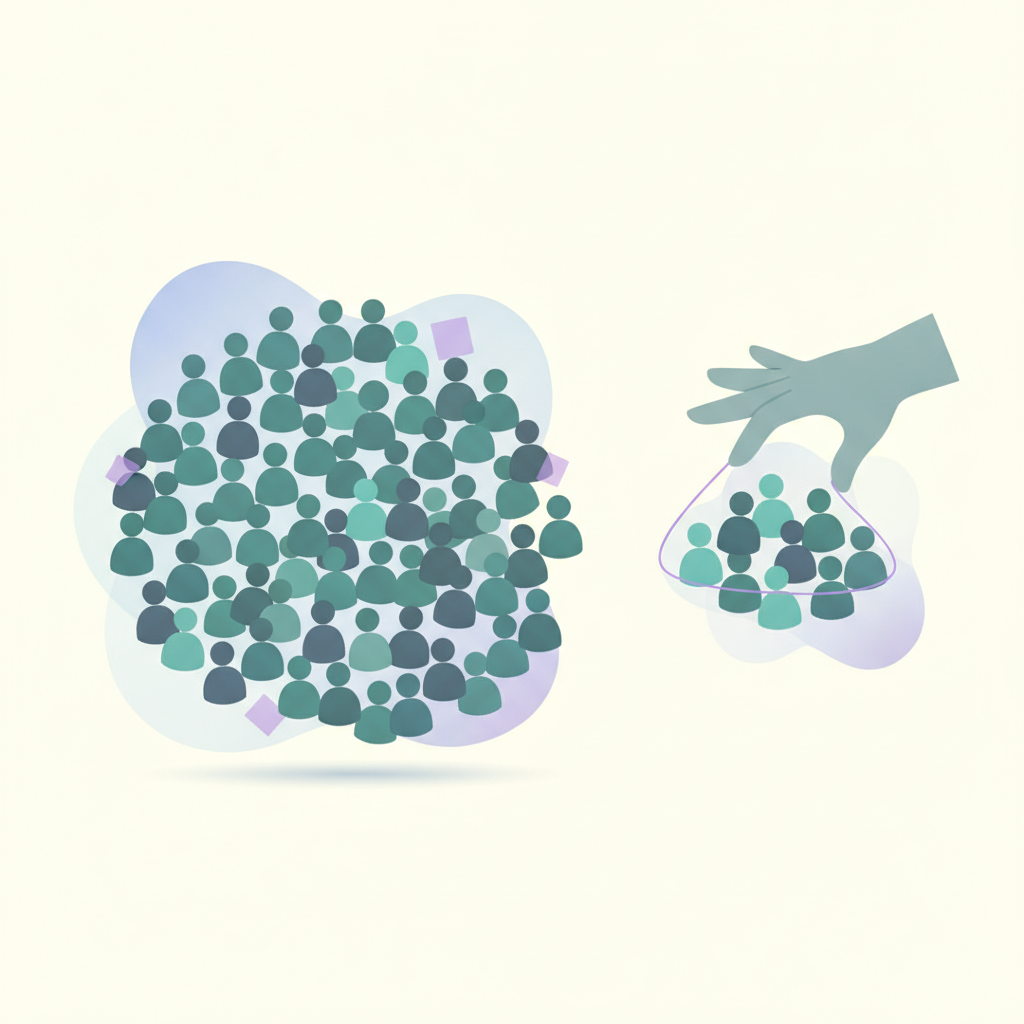
You can rarely measure everyone
Suppose you want the average commute time of every worker in a city. There are millions of them, they change jobs, and nobody has time to ask them all. Measuring the entire group is almost never possible — too expensive, too slow, sometimes physically impossible (you cannot test every light bulb by burning it out).
So statistics does something clever: it measures a small slice, then reasons carefully back to the whole. Getting that reasoning right starts with naming the two groups precisely.
Two words for a number: parameter vs statistic
Once you have a population and a sample, you will compute the same kinds of numbers — an average, a spread — for each. They get different names and different symbols so nobody confuses the true value with the estimate.
- A number that describes the population is a parameter. It is usually unknown and fixed. The population mean is \( \mu \) ("mu") and the population standard deviation is \( \sigma \) ("sigma").
- A number computed from your sample is a statistic. You can actually calculate it, and it changes from sample to sample. The sample mean is \( \bar{x} \) ("x-bar") and the sample standard deviation is \( s \).
A handy memory hook: parameter goes with population; statistic goes with sample. Greek letters describe the unknown truth; ordinary letters describe what you measured.
Watch a sample stand in for a population
The simulation below draws samples from a population whose true shape is fixed. The top strip is the whole population. Each time you draw, a handful of values is pulled out and its average recorded in the bottom panel.
For this lesson, focus on one idea: a single sample's average lands near the population mean but rarely exactly on it, and different samples give slightly different averages. That wobble — the fact that a statistic like \( \bar{x} \) changes from sample to sample — is exactly what the next lessons on sampling distributions are about.
The trap: sampling bias
A sample fails when it is systematically unlike the population — that is sampling bias. Bias is not the same as bad luck; it is a lean in one direction that repeats no matter how much data you collect.
The most common culprit is a convenience sample — grabbing whoever is easy to reach. Ask about commute times only in the office parking lot at 9am and you miss everyone who works from home, takes the train, or starts at noon. Poll about a product only among people who already follow your brand and you hear mostly fans. The sample is easy to get and quietly skewed.
The fix: random sampling
The cure is to remove your choices from the selection. In a simple random sample, every member of the population has an equal chance of being picked, and picks do not depend on who you find convenient. Randomness has no agenda, so on average the sample mirrors the population — fast and slow commuters show up in roughly their true proportions.
Random selection does more than remove bias. Because the picks are random, the sample statistic behaves in a predictable, mathematical way from sample to sample. That predictable behavior — the sampling distribution — is what lets statistics attach honest margins of error to an estimate, and it is exactly where the next lessons go.
- Population: all customers of the cafe — the group the manager actually cares about.
- Sample: the 40 early-Monday customers whose spend was recorded.
- The sample average is the statistic \( \bar{x} \); it is being used to estimate the population parameter \( \mu \), the true average spend of all customers.
- This is a convenience sample taken at one time of day. Early-morning customers may buy mostly coffee, while lunch and afternoon customers spend more on food — so the sample systematically leans low.
- The fix is not simply more early-morning customers; it is a random sample spread across times and days so every customer type has a fair chance to appear.
Check your understanding
- A population is the entire group you care about; a sample is the smaller subset you actually measure because studying everyone is usually impossible.
- A parameter describes the population (mean mu, standard deviation sigma) and is usually unknown; a statistic describes the sample (mean x-bar, standard deviation s) and is what you compute.
- We use sample statistics to estimate population parameters, so the sample must resemble the population in miniature.
- Sampling bias is a systematic lean toward one kind of member; convenience samples (whoever is easy to reach) are a classic cause, and a bigger sample does not fix it.
- Random sampling, where every member has an equal chance of selection, removes that lean and makes the statistic behave predictably — setting up sampling distributions.
🎓 Go deeper: external courses & trusted references
External sites are listed for reference only. This course is independent and has no affiliation with, or endorsement from, the institutions named.