
Bayes' Theorem & Base Rates
How to flip a conditional — and why a rare condition can turn even a strong test into a false-alarm machine.
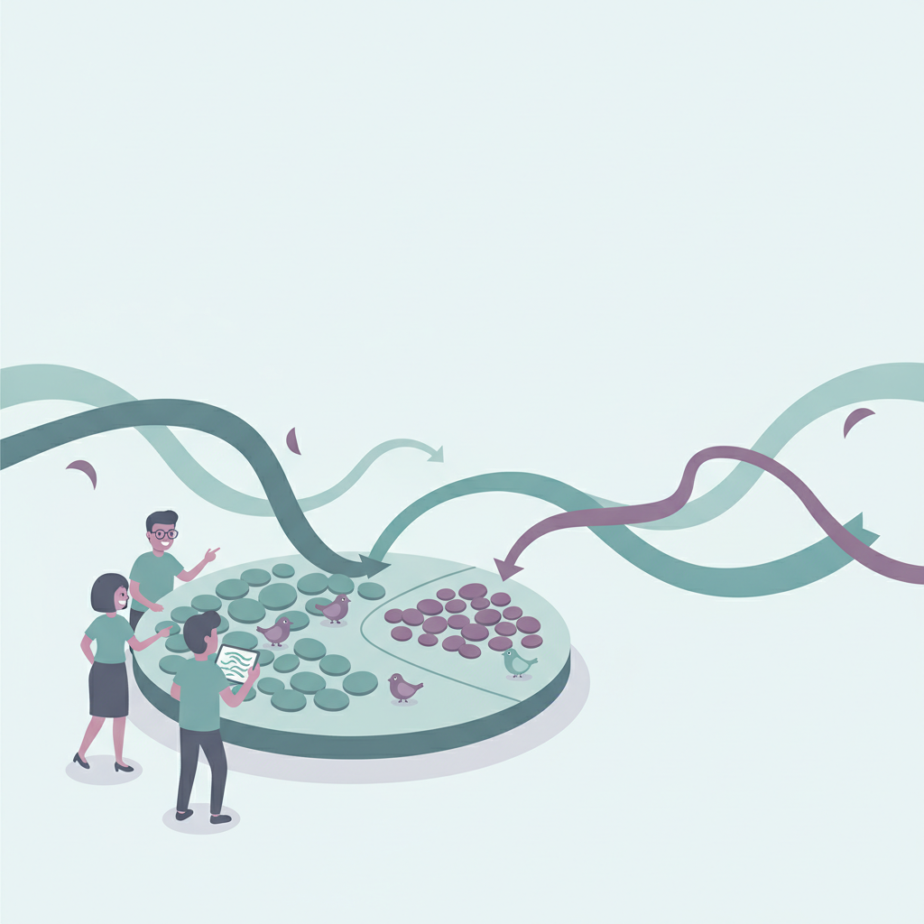
A positive result flips the question
Imagine a screening test for a rare condition. The lab says the test is 90% accurate, and your result comes back positive. It is tempting to conclude there is a 90% chance you have the condition. That feeling is almost always wrong — and the gap between it and the truth is one of the most useful ideas in probability.
The trap is that 90% accurate describes \(P(\text{positive}\mid\text{have it})\): among people who have the condition, how often the test fires. But what you want to know is the reverse — \(P(\text{have it}\mid\text{positive})\): among people who test positive, how many truly have it. These are not the same number, and Bayes' theorem is the tool for turning one into the other.
Bayes' theorem
Bayes' theorem stitches three quantities together:
- The base rate \(P(A)\) — often called the prior — how common the condition is before any test.
- The likelihood \(P(B\mid A)\) — how strongly the evidence B points to A (here, the test's true-positive rate).
- The overall chance of the evidence \(P(B)\) — how often a positive shows up at all, counting both true and false positives.
Put together, they give the flipped conditional you actually want:
The base-rate fallacy
Here is the heart of it. Suppose a condition affects just 1 in 100 people, and a test is 90% sensitive (catches 90% of real cases) and 92% specific (correctly clears 92% of healthy people). Those sound like strong numbers. Yet because 99 out of every 100 people are healthy, even a modest 8% false-positive rate on that huge healthy group produces a stack of false alarms — often more than the true positives from the tiny group who really have it.
Jumping straight from positive to I have it — while ignoring how rare the condition is — is the base-rate fallacy. The simulation below makes the pile of false positives impossible to miss. Drag prevalence down toward 1% and watch the red false-positive icons swamp the green true-positive ones, while the readout P(have it | positive) sinks far below the test's accuracy.
Count people, not percentages
These problems get dramatically easier if you stop juggling percentages and instead picture a concrete crowd — say 1,000 people — and count heads. This trick is called using natural frequencies, and it turns Bayes' theorem into simple arithmetic you can do without the formula.
- Start with 1,000 people. A 1% base rate means about 10 truly have the condition and 990 do not.
- True positives: 99% of the 10 who have it test positive — about 10 people.
- False positives: the test wrongly flags 5% of the 990 healthy people — about \(0.05 \times 990 \approx\) 50 people.
- Everyone who tests positive: \(10 + 50 = 60\) people, but only 10 of them truly have the condition.
- Flip the conditional: \(P(\text{have it}\mid\text{positive}) = \dfrac{10}{60} \approx 0.167\).
Check your understanding
- P(A|B) is generally not the same as P(B|A); Bayes' theorem is the rule that converts one into the other.
- Bayes weights the likelihood by the base rate (prior), so rare things stay fairly rare even after a positive test.
- The base-rate fallacy: ignore how common the condition is and you will badly overestimate P(have it | positive).
- With a rare condition, a small false-positive rate on a huge healthy group produces more false positives than true positives.
- Natural frequencies — counts out of 1,000 people — make these problems far easier than juggling percentages.
🎓 Go deeper: external courses & trusted references
External sites are listed for reference only. This course is independent and has no affiliation with, or endorsement from, the institutions named.